今さら言語処理100本ノック #7

他の 100 本ノックシリーズ

言語処理 100 本ノック(第 7 章: 単語ベクトル)

60. 単語ベクトルの読み込みと表示

Google News データセット（約 1,000 億単語）での学習済み単語ベクトル（300 万単語・フレーズ，300 次元）をダウンロードし，”United States”の単語ベクトルを表示せよ．ただし，”United States”は内部的には”United_States”と表現されていることに注意せよ．

ファイルサイズが1.5GBもあってやばいのでGoogle Colabなどを使うことをお勧めします。

ファイルダウンロード(Google colab)

%%bash
url="https://drive.google.com/uc?export=download&id=0B7XkCwpI5KDYNlNUTTlSS21pQmM"
curl -sc /tmp/cookie ${url} >/dev/null
code="$(awk '/_warning_/ {print $NF}' /tmp/cookie)"
curl -sLb /tmp/cookie ${url}"&confirm=${code}" -o GoogleNews-vectors-negative300.bin.gz

一応 sha256 も載せておく

! sha256sum GoogleNews-vectors-negative300.bin.gz
21c05ae916a67a4da59b1d006903355cced7de7da1e42bff9f0504198c748da8  GoogleNews-vectors-negative300.bin.gz

メイン

from gensim.models import KeyedVectors
model = KeyedVectors.load_word2vec_format('GoogleNews-vectors-negative300.bin.gz', binary=True)

model["United_States"]

array([-3.61328125e-02, -4.83398438e-02,  2.35351562e-01,  1.74804688e-01,
       -1.46484375e-01, -7.42187500e-02, -1.01562500e-01, -7.71484375e-02,
        1.09375000e-01, -5.71289062e-02, -1.48437500e-01, -6.00585938e-02,
        1.74804688e-01, -7.71484375e-02,  2.58789062e-02, -7.66601562e-02,
       -3.80859375e-02,  1.35742188e-01,  3.75976562e-02, -4.19921875e-02,
       -3.56445312e-02,  5.34667969e-02,  3.68118286e-04, -1.66992188e-01,
       -1.17187500e-01,  1.41601562e-01, -1.69921875e-01, -6.49414062e-02,
       -1.66992188e-01,  1.00585938e-01,  1.15722656e-01, -2.18750000e-01,
       -9.86328125e-02, -2.56347656e-02,  1.23046875e-01, -3.54003906e-02,
       -1.58203125e-01, -1.60156250e-01,  2.94189453e-02,  8.15429688e-02,
        6.88476562e-02,  1.87500000e-01,  6.49414062e-02,  1.15234375e-01,
       -2.27050781e-02,  3.32031250e-01, -3.27148438e-02,  1.77734375e-01,
       -2.08007812e-01,  4.54101562e-02, -1.23901367e-02,  1.19628906e-01,
        7.44628906e-03, -9.03320312e-03,  1.14257812e-01,  1.69921875e-01,
       -2.38281250e-01, -2.79541016e-02, -1.21093750e-01,  2.47802734e-02,
        7.71484375e-02, -2.81982422e-02, -4.71191406e-02,  1.78222656e-02,
       -1.23046875e-01, -5.32226562e-02,  2.68554688e-02, -3.11279297e-02,
       -5.59082031e-02, -5.00488281e-02, -3.73535156e-02,  1.25976562e-01,
        5.61523438e-02,  1.51367188e-01,  4.29687500e-02, -2.08007812e-01,
       -4.78515625e-02,  2.78320312e-02,  1.81640625e-01,  2.20703125e-01,
       -3.61328125e-02, -8.39843750e-02, -3.69548798e-05, -9.52148438e-02,
       -1.25000000e-01, -1.95312500e-01, -1.50390625e-01, -4.15039062e-02,
        1.31835938e-01,  1.17675781e-01,  1.91650391e-02,  5.51757812e-02,
       -9.42382812e-02, -1.08886719e-01,  7.32421875e-02, -1.15234375e-01,
        8.93554688e-02, -1.40625000e-01,  1.45507812e-01,  4.49218750e-02,
       -1.10473633e-02, -1.62353516e-02,  4.05883789e-03,  3.75976562e-02,
       -6.98242188e-02, -5.46875000e-02,  2.17285156e-02, -9.47265625e-02,
        4.24804688e-02,  1.81884766e-02, -1.73339844e-02,  4.63867188e-02,
       -1.42578125e-01,  1.99218750e-01,  1.10839844e-01,  2.58789062e-02,
       -7.08007812e-02, -5.54199219e-02,  3.45703125e-01,  1.61132812e-01,
       -2.44140625e-01, -2.59765625e-01, -9.71679688e-02,  8.00781250e-02,
       -8.78906250e-02, -7.22656250e-02,  1.42578125e-01, -8.54492188e-02,
       -3.18359375e-01,  8.30078125e-02,  6.34765625e-02,  1.64062500e-01,
       -1.92382812e-01, -1.17675781e-01, -5.41992188e-02, -1.56250000e-01,
       -1.21582031e-01, -4.95605469e-02,  1.20117188e-01, -3.83300781e-02,
        5.51757812e-02, -8.97216797e-03,  4.32128906e-02,  6.93359375e-02,
        8.93554688e-02,  2.53906250e-01,  1.65039062e-01,  1.64062500e-01,
       -1.41601562e-01,  4.58984375e-02,  1.97265625e-01, -8.98437500e-02,
        3.90625000e-02, -1.51367188e-01, -8.60595703e-03, -1.17675781e-01,
       -1.97265625e-01, -1.12792969e-01,  1.29882812e-01,  1.96289062e-01,
        1.56402588e-03,  3.93066406e-02,  2.17773438e-01, -1.43554688e-01,
        6.03027344e-02, -1.35742188e-01,  1.16210938e-01, -1.59912109e-02,
        2.79296875e-01,  1.46484375e-01, -1.19628906e-01,  1.76757812e-01,
        1.28906250e-01, -1.49414062e-01,  6.93359375e-02, -1.72851562e-01,
        9.22851562e-02,  1.33056641e-02, -2.00195312e-01, -9.76562500e-02,
       -1.65039062e-01, -2.46093750e-01, -2.35595703e-02, -2.11914062e-01,
        1.84570312e-01, -1.85546875e-02,  2.16796875e-01,  5.05371094e-02,
        2.02636719e-02,  4.25781250e-01,  1.28906250e-01, -2.77099609e-02,
        1.29882812e-01, -1.15722656e-01, -2.05078125e-02,  1.49414062e-01,
        7.81250000e-03, -2.05078125e-01, -8.05664062e-02, -2.67578125e-01,
       -2.29492188e-02, -8.20312500e-02,  8.64257812e-02,  7.61718750e-02,
       -3.66210938e-02,  5.22460938e-02, -1.22070312e-01, -1.44042969e-02,
       -2.69531250e-01,  8.44726562e-02, -2.52685547e-02, -2.96630859e-02,
       -1.68945312e-01,  1.93359375e-01, -1.08398438e-01,  1.94091797e-02,
       -1.80664062e-01,  1.93359375e-01, -7.08007812e-02,  5.85937500e-02,
       -1.01562500e-01, -1.31835938e-01,  7.51953125e-02, -7.66601562e-02,
        3.37219238e-03, -8.59375000e-02,  1.25000000e-01,  2.92968750e-02,
        1.70898438e-01, -9.37500000e-02, -1.09375000e-01, -2.50244141e-02,
        2.11914062e-01, -4.44335938e-02,  6.12792969e-02,  2.62451172e-02,
       -1.77734375e-01,  1.23046875e-01, -7.42187500e-02, -1.67968750e-01,
       -1.08886719e-01, -9.04083252e-04, -7.37304688e-02,  5.49316406e-02,
        6.03027344e-02,  8.39843750e-02,  9.17968750e-02, -1.32812500e-01,
        1.22070312e-01, -8.78906250e-03,  1.19140625e-01, -1.94335938e-01,
       -6.64062500e-02, -2.07031250e-01,  7.37304688e-02,  8.93554688e-02,
        1.81884766e-02, -1.20605469e-01, -2.61230469e-02,  2.67333984e-02,
        7.76367188e-02, -8.30078125e-02,  6.78710938e-02, -3.54003906e-02,
        3.10546875e-01, -2.42919922e-02, -1.41601562e-01, -2.08007812e-01,
       -4.57763672e-03, -6.54296875e-02, -4.95605469e-02,  2.22656250e-01,
        1.53320312e-01, -1.38671875e-01, -5.24902344e-02,  4.24804688e-02,
       -2.38281250e-01,  1.56250000e-01,  5.83648682e-04, -1.20605469e-01,
       -9.22851562e-02, -4.44335938e-02,  3.61328125e-02, -1.86767578e-02,
       -8.25195312e-02, -8.25195312e-02, -4.05273438e-02,  1.19018555e-02,
        1.69921875e-01, -2.80761719e-02,  3.03649902e-03,  9.32617188e-02,
       -8.49609375e-02,  1.57470703e-02,  7.03125000e-02,  1.62353516e-02,
       -2.27050781e-02,  3.51562500e-02,  2.47070312e-01, -2.67333984e-02],
      dtype=float32)

61. 単語の類似度

“United States”と”U.S.”のコサイン類似度を計算せよ．

genisum のビルドインを使う

参考: gensim: models.deprecated.word2vec – Deep learning with word2vec

model.similarity("U.S.", "United_States") #> 0.73107743

numpy で頑張る

import numpy as np
def cos_sim(v1, v2):
    """2ベクトル間のコサイン類似度を返す"""
    return np.dot(v1, v2) / (np.linalg.norm(v1) * np.linalg.norm(v2))

cos_sim(model["United_States"], model["U.S."]) #> 0.7310775

62. 類似度の高い単語 10 件

“United States”とコサイン類似度が高い 10 語と，その類似度を出力せよ．

model.most_similar_cosmul("United_States")

[('Unites_States', 0.8938615918159485),
 ('Untied_States', 0.8770676851272583),
 ('United_Sates', 0.8700354099273682),
 ('U.S.', 0.8655378818511963),
 ('theUnited_States', 0.8202189207077026),
 ('America', 0.8089197278022766),
 ('UnitedStates', 0.8083648085594177),
 ('Europe', 0.8066486716270447),
 ('countries', 0.8022394776344299),
 ('Canada', 0.8009527325630188)]

63. 加法構成性によるアナロジー

“Spain”の単語ベクトルから”Madrid”のベクトルを引き，”Athens”のベクトルを足したベクトルを計算し，そのベクトルと類似度の高い 10 語とその類似度を出力せよ．

[('Greece', 0.9562304615974426),
 ('Aristeidis_Grigoriadis', 0.8694582581520081),
 ('Ioannis_Drymonakos', 0.8600285053253174),
 ('Ioannis_Christou', 0.8544448614120483),
 ('Greeks', 0.8521003127098083),
 ('Hrysopiyi_Devetzi', 0.8383888006210327),
 ('Panagiotis_Gionis', 0.8323913216590881),
 ('Heraklio', 0.8297829627990723),
 ('Lithuania', 0.8291547298431396),
 ('Periklis_Iakovakis', 0.8289119601249695)]

おまけ

[('Japan', 1.0016356706619263),
 ('Japanese', 0.8822101950645447),
 ('South_Korea', 0.8762961626052856),
 ('Korea', 0.8596336245536804),
 ('Japans', 0.8564624190330505),
 ('Shimane_Prefecture', 0.8264696598052979),
 ('Nagasaki_Prefecture', 0.824508011341095),
 ('Kyushu', 0.8202904462814331),
 ('Kanto_region', 0.8149427771568298),
 ('Takao', 0.8107433915138245)]

64. アナロジーデータでの実験

単語アナロジーの評価データをダウンロードし，vec(2 列目の単語) - vec(1 列目の単語) + vec(3 列目の単語)を計算し，そのベクトルと類似度が最も高い単語と，その類似度を求めよ．求めた単語と類似度は，各事例の末尾に追記せよ．

ダウンロード

curl -O http://download.tensorflow.org/data/questions-words.txt

メイン

with open("questions-words.txt") as f:
  lines = f.readlines()

def solve(lines):
  for line in lines:
    if line.startswith(":"):
      yield line
      continue

    cols = line.rstrip("\n").split()
    if len(cols) != 4:
      yield line
      continue

    word, _ = model.most_similar_cosmul(positive=cols[1:3], negative=cols[0:1])[0]
    yield "{} {} {} {} {}\n".format(*cols, word)

with open("questions-words.txt.v1", mode='x') as f:
  for e in solve(lines):
    f.write(e)

Google Colab で寝ているときに回していたけど、多分 7 時間くらいかかった。

19558 行 x1s で 5 時間半くらいなので 1 行 1 秒ちょっとの時間がかかっている。

$ awk 'NR % 500 == 0' questions-words.txt.v1
Tokyo Japan Madrid Spain Spain
Baku Azerbaijan Dhaka Bangladesh Bangladesh
Bucharest Romania Georgetown Guyana Villanova
Dublin Ireland Jakarta Indonesia Indonesia
Kathmandu Nepal Kigali Rwanda Rwanda
Lusaka Zambia Tashkent Uzbekistan Uzbekistan
Nassau Bahamas Tokyo Japan Japan
Rome Italy Vientiane Laos Laos
Thimphu Bhutan Abuja Nigeria Nigeria
Zagreb Croatia Apia Samoa Samoa
Latvia lats Nigeria naira naira
Philadelphia Pennsylvania Cleveland Ohio Ohio
Louisville Kentucky Lubbock Texas Texas
Wichita Kansas Irving Texas lawyer_Elmar_Kresbach
Orlando Florida Worcester Massachusetts Massachusetts
Modesto California Miami Florida Florida
grandfather grandmother father mother mother
complete completely efficient efficiently inefficient
quiet quietly serious seriously already
comfortable uncomfortable rational irrational irrational
possibly impossibly decided undecided unadorned
fast faster bright brighter brighter
safe safer heavy heavier heavier
young younger safe safer safer
low lowest cool coolest coolest
warm warmest strange strangest strangest
increase increasing scream screaming screaming
sit sitting shuffle shuffling shuffling
Cambodia Cambodian Ukraine Ukrainian Ukrainian
Ireland Irish Brazil Brazilian Brazilian
Portugal Portuguese Croatia Croatian Croatian
feeding fed looking looked hoping
paying paid running ran ran
sleeping slept selling sold sold
car cars cat cats cats
eye eyes donkey donkeys donkeys
pig pigs machine machines machines
listen listens eat eats eats
walk walks vanish vanishes vanishes

memo

並列処理しようとしてうまくいかなかった

Python の並列処理・並行処理をしっかり調べてみた - Qiita

def solve(index, lines):
  line = lines[index]
  if line.startswith(":"):
    lines[index] =  line
    return

  cols = line.rstrip("\n").split()
  if len(cols) != 4:
    lines[index] =  line
    return

  word, _ = model.most_similar_cosmul(positive=cols[1:3], negative=cols[0:1])[0]
  lines[index] =  "{} {} {} {} {}\n".format(*cols, word)
  return

# 並列処理
from multiprocessing import Process, Manager
ll = lines[:30]
manager = Manager()
returned = manager.list(ll)

for i in range(len(ll)):
  process = Process(
      target=solve,
      kwargs={
          "index":i,
          'lines': returned,
      })

  process.start()
  process_list.append(process)

for process in process_list:
    process.join()

# 通常処理
ll = lines[:30]
for i in range(len(ll)):
  solve(i, ll)

print(ll == list(returned)) #> True

並列処理と通常処理の timeit 結果はそれぞれ1 loop, best of 3: 36 s per loop, 1 loop, best of 3: 30.4 s per loop

期待する返り値は得られているけど、実行速度がむしろ遅くなってる。並行処理わからんぞ;(

65. アナロジータスクでの正解率

64 の実行結果を用い，意味的アナロジー（semantic analogy）と文法的アナロジー（syntactic analogy）の正解率を測定せよ．

最初何を言っているのかわからなかったのですが、どうやら意味的アナロジーと文法的アナロジーはquestions-words.txtにおける分類のようです。

$ cat questions-words.txt | grep ":"
: capital-common-countries
: capital-world
: currency
: city-in-state
: family
: gram1-adjective-to-adverb
: gram2-opposite
: gram3-comparative
: gram4-superlative
: gram5-present-participle
: gram6-nationality-adjective
: gram7-past-tense
: gram8-plural
: gram9-plural-verbs

カテゴリ名にgramが含まれるものを文法的アナロジー, そうでないものを意味的アナロジーとします。

メイン

import numpy as np

with open("questions-words.txt.v1") as f:
  lines = f.readlines()

semantic, syntactic = [], []
for line in lines:
  if line.startswith(": gram"):
    ctg =  "syntactic"
  elif line.startswith(":"):
    ctg =  "semantic"
  else:
    if ctg == "semantic":
      semantic.append(line.rstrip("\n").split())
    if ctg == "syntactic":
      syntactic.append(line.rstrip("\n").split())


def calc(data):
  """data: List[List[str]{5}]"""
  ndarray = np.array(data)
  ans, prd = ndarray[:, 3:5].T
  return np.mean(ans==prd)

print("semantic: ", calc(semantic)) #> semantic:  0.7411207576953434
print("syntactic: ", calc(syntactic)) #> syntactic:  0.7600936768149883

文法的アナロジーの方が正答率は良さげですね。

66. WordSimilarity-353 での評価

The WordSimilarity-353 Test Collectionの評価データをダウンロードし，単語ベクトルにより計算される類似度のランキングと，人間の類似度判定のランキングの間のスピアマン相関係数を計算せよ．

python で相関係数の計算をする | Monotalk

$ curl -s http://www.gabrilovich.com/resources/data/wordsim353/wordsim353.zip -o wordsim353.zip
$ unzip wordsim353.zip

with open("combined.tab") as f:
  lines = f.readlines()

def nlp100_66_pre(lines):
  for line in lines:
    w1, w2, human = line.rstrip("\n").split("\t")
    if (w1 in model and w1 in model):
      vec = model.similarity(w1, w2)
      yield np.float32(human), vec

score = nlp100_66_pre(lines[1:])
human, vec = np.array(list(score)).T
from scipy.stats import spearmanr

correlation, pvalue = spearmanr(human, vec)
print("相関係数", correlation) #> 相関係数 0.7000166486272194
print("p値", pvalue) #> p値 2.86866666051422e-53

67. k-means クラスタリング

国名に関する単語ベクトルを抽出し，k-means クラスタリングをクラスタ数 k=5 として実行せよ．

国名を収集する, 単語ベクトル化

questions-words.txtのカテゴリcapital-common-countries, capital-worldから国名を収集する。

with open("questions-words.txt") as f:
  lines = f.readlines()

cots = []
for line in lines:
  if line.startswith(": currency"):
    break
  elif line.startswith(":"):
    continue
  else:
    _, a, _, b = line.rstrip("\n").split()
    cots += [a, b]

dct = {}
for e in set(cots):
  if e in model:
    dct[e] = model[e]

sklearn KMeans でクラスタリング

from sklearn.cluster import KMeans
pred = KMeans(n_clusters=5).fit_predict(list(dct.values()))

print([list(dct.keys())[i] for i, p in enumerate(pred) if p == 0])
#> ['Suriname', 'Nepal', 'Tuvalu', 'Peru', 'Thailand', 'Jamaica', 'Honduras', 'China', 'Dominica', 'Vietnam', 'Fiji', 'Indonesia', 'Bangladesh', 'Bhutan', 'Australia', 'Samoa', 'Guyana', 'Japan', 'Venezuela', 'Cuba', 'Canada', 'Laos', 'Philippines', 'Bahamas', 'Uruguay', 'Belize', 'Nicaragua', 'Chile', 'Ecuador', 'Taiwan']

日本が属するラベルは東南アジアと島国という特徴が出ていますね。

from collections import Counter
c = Counter(pred)
print(c) #> Counter({0: 30, 4: 27, 1: 25, 2: 19, 3: 15})

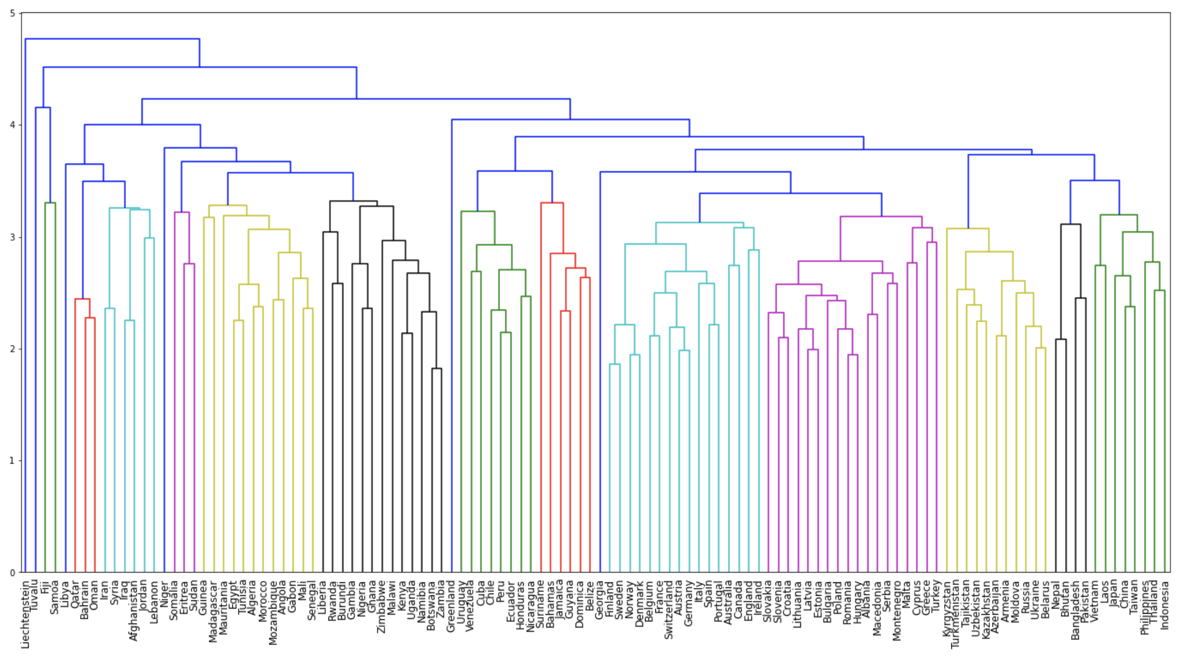
68. Ward 法によるクラスタリング

国名に関する単語ベクトルに対し，Ward 法による階層型クラスタリングを実行せよ．さらに，クラスタリング結果をデンドログラムとして可視化せよ．

from scipy.cluster.hierarchy import dendrogram, linkage
import matplotlib.pyplot as plt

plt.figure(figsize=(24, 12))
Z = linkage(list(dct.values()), method="weighted", metric="euclidean")
dendrogram(Z, labels=list(dct.keys()))
plt.xticks(fontsize=12)
plt.show()

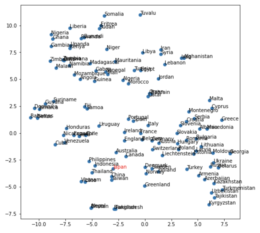
69. t-SNE による可視化

ベクトル空間上の国名に関する単語ベクトルを t-SNE で可視化せよ．

from sklearn.manifold import TSNE
tsne = TSNE()
tsne.fit(list(dct.values()))

TSNE(angle=0.5, early_exaggeration=12.0, init='random', learning_rate=200.0,
     method='barnes_hut', metric='euclidean', min_grad_norm=1e-07,
     n_components=2, n_iter=1000, n_iter_without_progress=300, n_jobs=None,
     perplexity=30.0, random_state=None, verbose=0)

plt.figure(figsize=(8, 8))
plt.scatter(tsne.embedding_[:, 0], tsne.embedding_[:, 1])
for (x, y), name in zip(tsne.embedding_, list(dct.keys())):
    if name == "Japan":
      plt.annotate(name, (x, y), color='r')
    else:
      plt.annotate(name, (x, y))
plt.show()